Linear Regression is one of simplest, basic algorithm you would wish to start your learning with. But let me remind you, the concept of linear regression is with us way before machine learning and AI caught our attention! I am sure you could recall studying its basic version in your high school or engineering mathematics or statistics class.
So let me share with you one simple scenario where linear regression comes into picture!
We are a family of two living in Bangalore city. Every day we approximately make 5 chapatis for dinner. I can cook them easily. Let’s say we purchased a house of our own here (Haha..In my dreams!).
Anyway, now every day either friends, colleagues or nosey relatives visit us to see our house and we courteously offer them to have dinner with us. Since I am new to cooking and I don’t want to be known as a bad host, every day I keep fretting about the availability of sufficient oil, ghee or flour once the guests arrive. How do I plan the dinner ahead? Once I know how many people are coming, I can try and estimate how many chapatis I’ll need to cook, can keep track of the required materials and be happy!
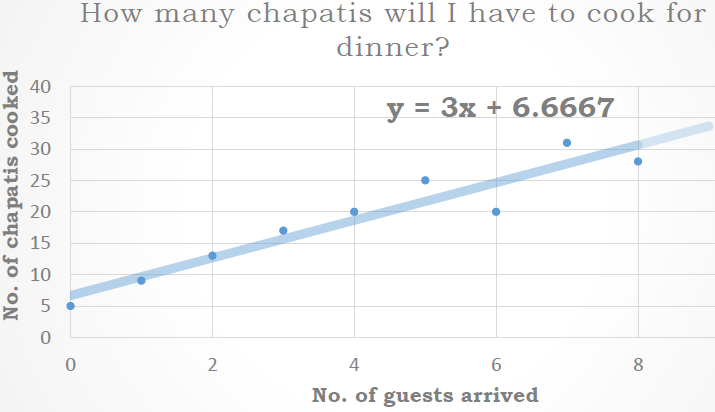
Figure (1) below shows my record of past 1 week.
What do we observe here?
Our data consists of two counts. One is the count of guests arriving and one is the count of chapatis I am cooking for dinner and both share a sort of linear relationship. So does the blue line shooting straight across the data points in the above X-Y plot ring any bell?? Yes, it is the “best-fit line” plotted to help us estimate approx. how many chapatis are cooked each day. It can help us find the number of chapatis required to be cooked any day in future based on the guests’ head count. Now plotting this line was easy on MS-PowerPoint. But what happens behind the scenes actually is called simple linear regression. This best-fit line tells that approximately in the absence of any guests arriving I’ll be cooking 6.66 chapatis, rounding up to 7 and in the presence of guests, I’ll need 3 chapatis per head. This best-fit line helps us in identifying the trend in the data.
Simple Linear Regression
In standard form, the “best-fit” line is given by ?=??+? where, ? is the slope of the line which tells us how the value of ? is linearly proportional to the value of ?, thus making ?, a dependent variable and ?, an independent variable. Here ? is the intercept which gives a value of ? in absence of any input value ?.
Calculation of ? and ?:
So how to find this “best-fit” line for the data given?
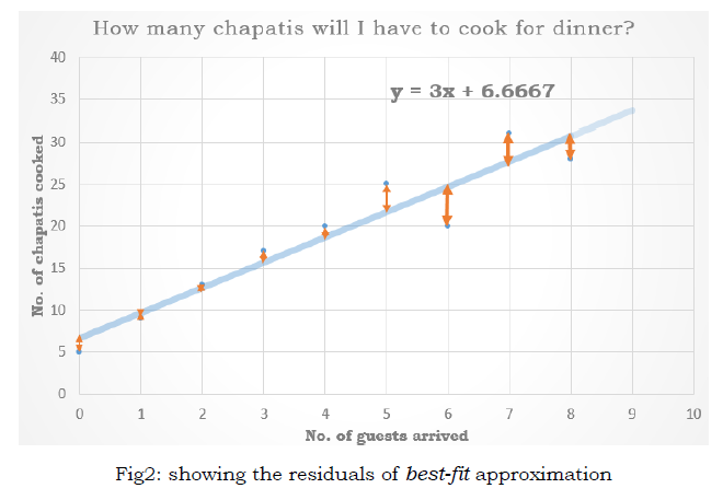
We can start with some random values (by an intelligent guess!) for ? and ? and plot an initial line. Then we compute the perpendicular distance of each point from the line, which is known as residual, difference between the true value of ? and the approximate value. It’s a no brainer that the residual should be as low as possible. Figure (2) shows the residual values marked by red lines. These values can be positive or negative and simply indicate the error in approximation. So we will minimize the sum of squares of residuals (cost) by changing values of ? and ? step-by-step. When the cost stops decreasing we fix that ? and ? as our final result. And this entire calculation can be done in excel sheet when we have only a bunch of data points.
In the simplest words, linear regression means inferring the relationship between dependent and independent variables. Using simple linear regression we knowingly or unknowingly take decisions or draw conclusions in our day-to-day life. For example, by estimating the salary for a new joiner based on the years of experience, estimating the commute-time based on the traffic in the area and weather conditions, estimating the availability of parking lot in a shopping center based on the day being a weekday, weekend or festival, sales of sarees during wedding season and festivals versus offseason. All these are the examples where linear regression can help make some estimation or inference based on the data gathered during the similar past events.
When linear regression gets used for machine learning, its dynamics changes because of the Big Data. To make a prediction about a certain event based on data in the range of thousands, obviously will make the computations more tedious and importance is given more to the predictive power of the algorithm than the underlying feature dependencies. Let’s look into that now.
Machine learning stands by its name. It is how a machine learns something useful and productive from the given data.
For a 3-5 year old boy buying chocolate is all about enjoying its taste. As he grows old and accompanies his father for chocolate shopping, he learns how his father pays more for bigger size chocolates or a large number of chocolates. It simply learns by observation and curiosity and soon he will learn how to buy chocolates for himself, how much to pay and all. Similarly, the computer needs to see and learn how one variable in the data is related to another one. For example, how the price of the house is related to the area of the house and number of bedrooms so that in future, it can predict the price of the house whose price data is not available to it earlier. The data it uses for learning is known as training data. And the data on which its learning is evaluated is known as test data. Now while teaching the machine, it needs to be given the “true answers” as well. This is known as supervised learning. It observes what it needs to learn. Linear regression algorithm comes under supervised machine learning because the algorithm needs both ? and ? variables to learn the relationship between them and find the best-fitting line.
Multiple Linear Regression
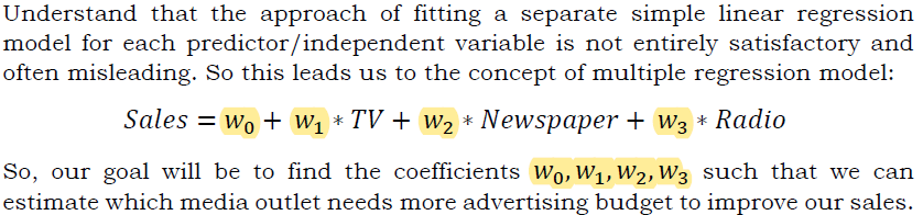
Earlier we saw how we can estimate one variable based on the other variable. What if a particular event is dependent on multiple variables? Simple. It can be solved by multiple linear regression. For example, you are estimating a yearly budget of advertising for your product sales. And you have different modes of advertisement like Radio, TV, and Newspaper. So how will you divide the budget? As a statistical consultant, you will have to answer various questions:
If there is any relationship between advertising budget and sales? And if so, how strong? Which media of the three, contributes the most to the produce sales? And if you find that there is any linear relationship between advertising expenses in media outlets and sales, then linear regression is an appropriate tool to use for advising the client about adjusting the advertising budgets, thereby indirectly improving sales. The figure below shows linear relationship between sales and advertisement media TV. Same we can analyze for Newspaper and Radio. So here we have 3 features/independent variables to take care of.
Observe the plot below for one variable:
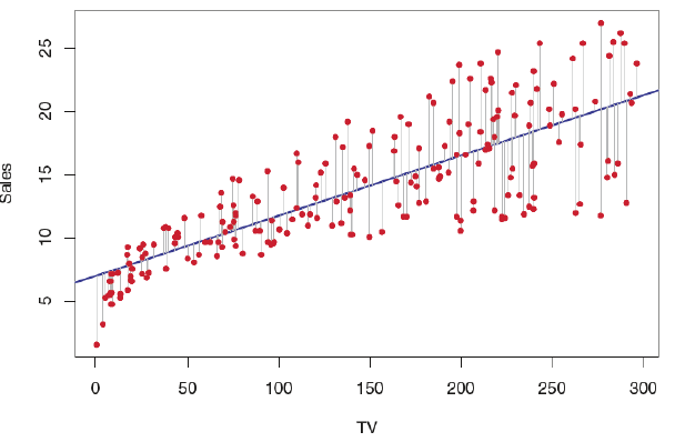
Fig3: Advertising data, best line fitting for the regression of sales onto TV for nearly 200 markets
General Equation for Linear Regression
Now you must have got a pretty good idea about linear regression in general and how it rules our world and helps statisticians and analysts make business decisions. So let’s talk about how to train a linear regression algorithm for supervised learning. Trust me, we can walk through it seamlessly!
For supervised learning we need to provide dataset of the following format:
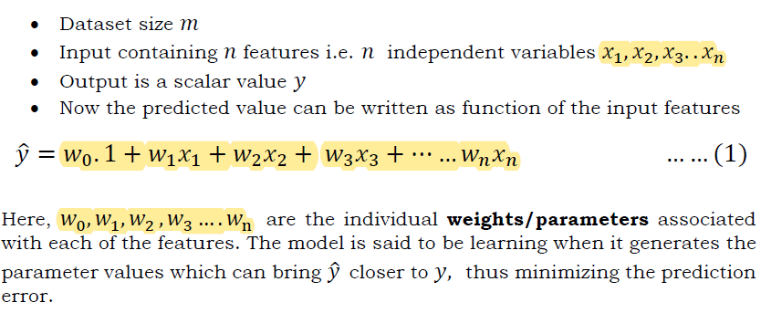
Equation (1) tells us how the weights/parameters determine the effect of features on the prediction. So if weight ?? is a very large value, then feature ?? will have larger impact on our prediction ?̂ and if ??=0 then the feature ?? will have no impact on our prediction ?̂. Similarly, if ?? is positive then ?̂ will be directly proportional to ?? and if ?? is negative then ?̂ will be inversely proportional to ??.
Now the model needs to learn from the data as to which features influence the target value and by how much and accordingly the weights are updated to reach at the targeted true value.
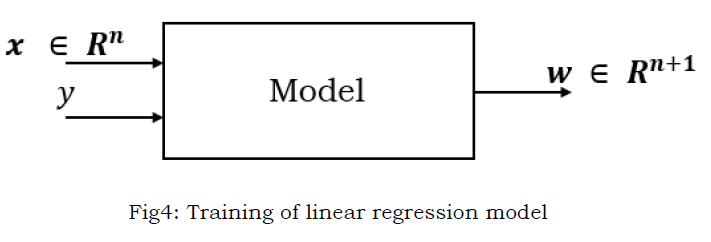
Figure (4) shows that supervised linear regression model takes in the dataset of the form (????? ????????,???? ?????? ?????) and determines appropriate model weights or parameters that can give most accurate prediction for the output.
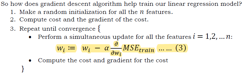
So how are these weights/parameters determined?
Remember the calculation of ? and ? we studied earlier? Something of that sort only!
We want the “predicted value ?̂” to be closer to the “true value ?”. So while learning if the residual (?̂(?)−?(?)), also known as the prediction error is more, the model should suffer a higher cost.
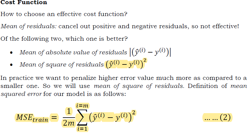
The goal of our model is to do whatever it takes to minimize the loss/cost it suffers. It has to reach a set of parameter values such that for the given data it can perform the best possible prediction. This process is known as model optimization.
One of the most popular algorithms which can minimize a function governed by a set of parameters is Gradient Descent.
Gradient Descent Algorithm
I know it sounds eccentric but its concept is very simple. Let’s understand it with an analogy.
Suppose you are on a mountain, exhausted after trekking on rough terrain. It’s dawn, there are fog and thin air. You wish to climb down, reach near the lake in the beautiful green valley. Since the visibility is poor you have to place your steps slowly and probably with the help of a stick or some kind of support. The best way is to measure the ground nearby and check where the land seems to descend and move in that direction. After every step, you will smartly calculate the direction like this and slowly and steadily reach the lake. Finally, you have fresh air, water and lots of greenery to soothe your eyes!
Now take the cost function and plot it with respect to model parameters. It will be some sort of peaks and valleys curve and your goal is to find the parameters where the cost function is minimum, so you have to reach the valley point in the curve. Look at the figure below for understanding in simpler terms.

Here, J represents the cost function and w represents the parameter
Bear with a little calculus concept!
The gradient of the cost function for a given point signifies the slope of the tangent to the curve at that point. The slope of the tangent gives us the direction of rising. Model’s idea is to reach the minimum so it moves in the opposite direction of the gradient.
Here, ? is real number called learning rate which signifies by how much the weight update is done.
Once the model processes through the entire training data, it has learned the optimal values of parameters and its performance can now be evaluated using the test data.
Of course, linear regression is an extremely simple and limited learning algorithm, but I hope that this article has got you curious about more such learning models, about how they work and how they can be trained with the help of a given data to later perform complex tasks. That was my goal. Happy Learning 🙂
Keep Coding 🙂
Vishwa Dadhania
The Data Monk services
We are well known for our interview books and have 70+ e-book across Amazon and The Data Monk e-shop page . Following are best-seller combo packs and services that we are providing as of now
- YouTube channel covering all the interview-related important topics in SQL, Python, MS Excel, Machine Learning Algorithm, Statistics, and Direct Interview Questions
Link – The Data Monk Youtube Channel - Website – ~2000 completed solved Interview questions in SQL, Python, ML, and Case Study
Link – The Data Monk website - E-book shop – We have 70+ e-books available on our website and 3 bundles covering 2000+ solved interview questions. Do check it out
Link – The Data E-shop Page - Instagram Page – It covers only Most asked Questions and concepts (100+ posts). We have 100+ most asked interview topics explained in simple terms
Link – The Data Monk Instagram page - Mock Interviews/Career Guidance/Mentorship/Resume Making
Book a slot on Top Mate
The Data Monk e-books
We know that each domain requires a different type of preparation, so we have divided our books in the same way:
1. 2200 Interview Questions to become Full Stack Analytics Professional – 2200 Most Asked Interview Questions
2.Data Scientist and Machine Learning Engineer -> 23 e-books covering all the ML Algorithms Interview Questions
3. 30 Days Analytics Course – Most Asked Interview Questions from 30 crucial topics
You can check out all the other e-books on our e-shop page – Do not miss it
For any information related to courses or e-books, please send an email to nitinkamal132@gmail.com